Neural Networks

From Biological Inspiration to Mathematical Foundation

Dr. Dhaval Patel • 2025

🎯 Complete Learning Journey

Here, we will learn from a neural network from beginner to someone who truly understands it.

🧠 Motivation

Neural networks power everything from your smartphone's camera to autonomous vehicles. Understanding them isn't just academic—it's essential for anyone working in modern technology.

Fundamental Challenge: Why traditional programming fails at pattern recognition
Biological Inspiration: How brain-like structures solve impossible problems
Mathematical Foundation: The elegant math that makes it all work
Practical Implementation: From theory to working code
Advanced Concepts: Weight optimization and learning algorithms
Real-World Applications: How these concepts scale to modern AI

Part I

The Fundamental Challenge

The Human-Computer Paradox

A cartoon π character looks at three variations of the handwritten digit '3', highlighting the concept that humans can generalize different styles of the same digit, a task neural networks aim to mimic.

🤔 The Paradox

For Humans: Instant, effortless, automatic recognition across infinite variations.

For Computers: Each pixel must be analyzed, patterns must be hard-coded, exceptions must be manually programmed.

⚠️ Traditional Approach Fails
Try writing an if-statement to recognize ANY handwritten "3" - you'll quickly realize it's impossible!

This is exactly why we need a fundamentally different approach: Neural Networks.

Traditional Programming vs Neural Networks

Traditional Programming

Rule-Based Approach:

Programmer writes explicit rules
If-then-else logic chains
Every scenario must be anticipated
Breaks down with complexity
Cannot handle exceptions gracefully

if (pixel[100] > 0.5 && pixel[101] > 0.5) {
// What goes here for "3"?
}

Neural Networks

Learning-Based Approach:

Network learns patterns from examples
Automatic feature extraction
Handles unseen variations
Scales with data complexity
Graceful degradation

Show 1000s of examples:
"This is a 3", "This is a 3"...
Network learns to recognize ANY 3!

VS

Part II

Understanding Neurons: The Building Blocks

🧠 Introduction: The "Neuron"

Let's understand what a neural network neuron actually is:

A neuron is simply: A container that holds a single number between 0.0 and 1.0

That's it. No complex biology, no mysterious processes. Just a number.

🔢 The "Activation" Concept

This number is called the neuron's activation:

0.0: Neuron is "off" or inactive
1.0: Neuron is "fully activated" or "fired up"
0.3, 0.7, etc.: Partial activation levels

🎯 Note: Think of neurons like dimmer switches for lights. Each can be off (0), fully on (1), or anywhere in between. The pattern of all these "light levels" across the network represents information.

Input Layer: Converting Reality to Numbers

Zoomed-in view of a grayscale image (digit '3') showing pixel values from 0.0 to 1.0, representing normalized intensity levels used as input for a neural network.

📊 The Conversion Process

Image → Numbers:

28×28 pixel image = 784 total pixels
Each pixel: brightness value 0.0-1.0
Black pixels = 0.0
White pixels = 1.0
Gray pixels = values between

28 × 28 = 784 input neurons

🔄 Information Encoding

Every piece of information must be converted to numbers between 0 and 1 to be processed by a neural network.

The Input Layer in Action

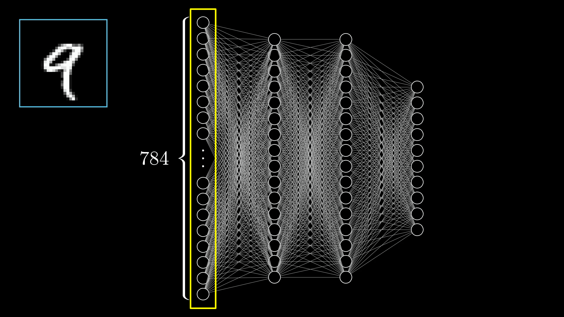
Same digit classification network with the first input layer highlighted in yellow, emphasizing the 784 input nodes corresponding to 28x28 image pixels.

🔍 Layer Breakdown

Input Layer Structure:

784 neurons total
Each neuron = one pixel
Organized in conceptual 28×28 grid
Values fed simultaneously

Critical Point: The network doesn't see "images" - it only sees 784 numbers! The spatial relationship must be learned.

                    Universal Principle: ANY input (text, audio, video) must be converted to numbers in this range.
                

Output Layer: Making Predictions

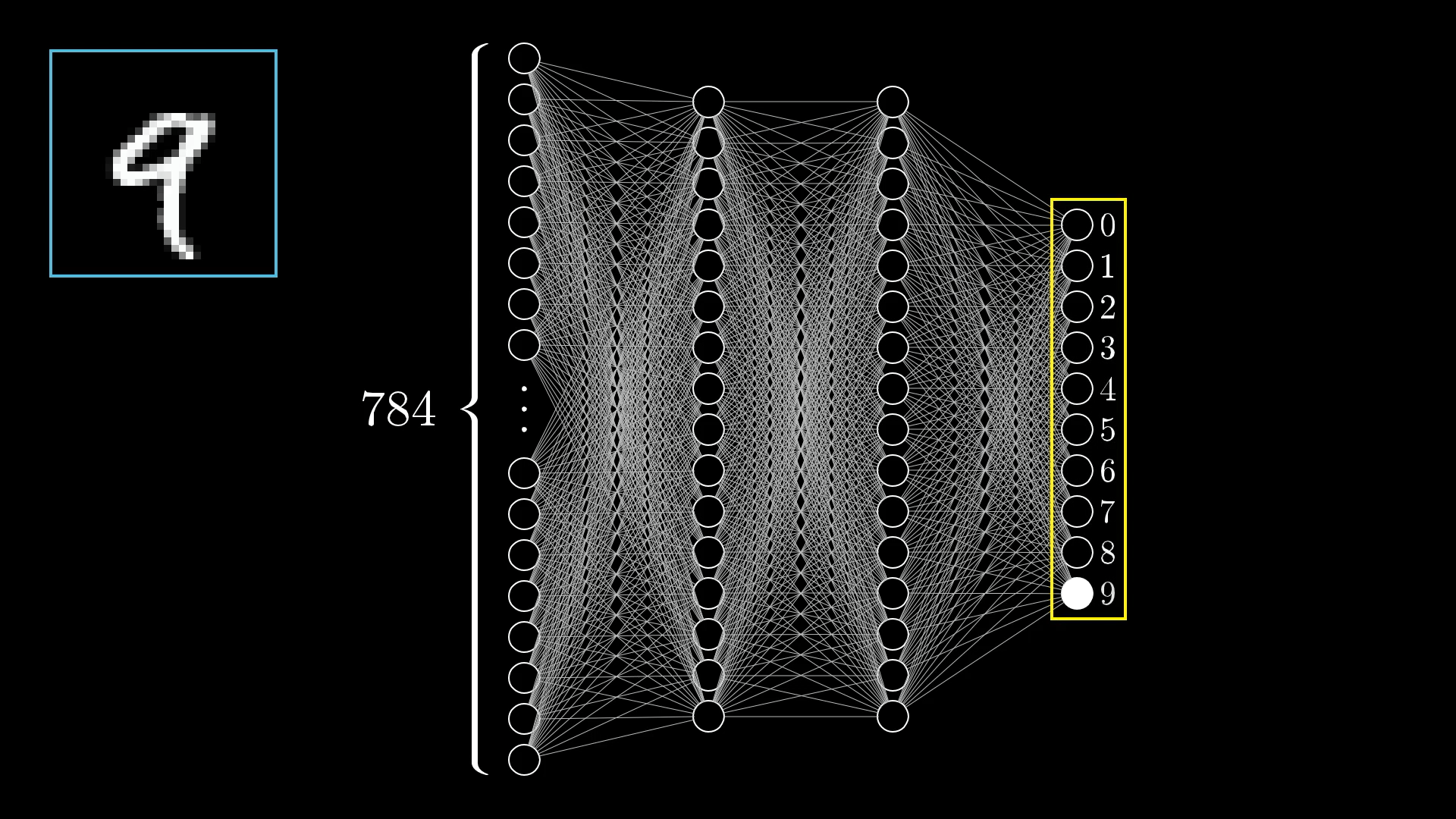
A feedforward neural network diagram for digit recognition using the MNIST dataset. The input is a handwritten digit '9', converted into 784 input neurons, followed by multiple hidden layers, and finally a 10-neuron output layer. The highlighted output neuron (index 9) indicates the model's prediction.

🎯 Prediction Mechanism

10 Output Neurons:

Neuron 0: "How much does this look like 0?"
Neuron 1: "How much does this look like 1?"
...
Neuron 9: "How much does this look like 9?"

Highest activation = Network's "best guess"

The beauty: Network can express uncertainty! Multiple neurons can be partially activated.

When Networks Are Uncertain

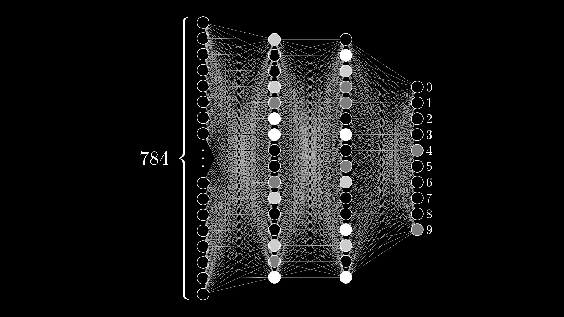
Digit classification neural network where multiple output nodes are activated with varying intensities. The output for '4' and '9' are darker, indicating uncertainty.

🤔 Interpreting Uncertainty

What This Tells Us:

Network is torn between "4" and "9"
Both neurons highly activated
Other digits have low confidence
This reflects realistic ambiguity!

🧠 Human-Like Reasoning

Just like humans might be unsure between similar-looking digits, networks can express this uncertainty through activation patterns.

🎯 Think About It: How would you decide if a handwritten digit is a 4 or a 9? The network faces the same challenge!

Part III

The Hidden Layers: Where Magic Happens

The Great Mystery: Hidden Layers

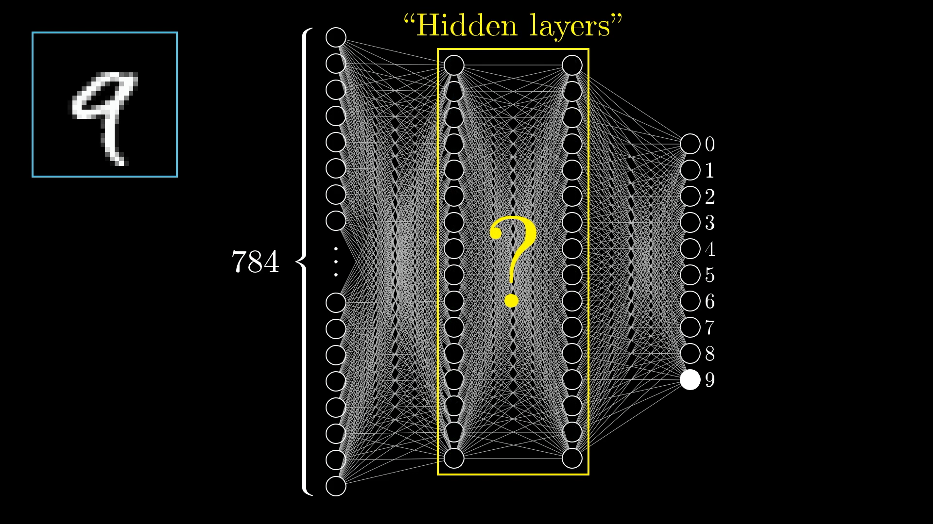
A neural network diagram with the hidden layers highlighted using a yellow box and question mark, symbolizing their mysterious role in feature learning.

❓ The Big Questions

What are these layers actually doing?
How do they transform 784 numbers into 10 predictions?
Why not connect input directly to output?

The Challenge: We have 784 inputs, 10 outputs, and need something powerful enough to recognize any digit pattern.

🔍 The Hypothesis

Hidden layers learn to detect increasingly complex features, building up from simple to sophisticated patterns.

The Hierarchical Learning Hypothesis

🏗️ Layer 1: Edge Detection

The first hidden layer learns to detect basic edges and simple patterns.

Pixels → Simple Edges

Horizontal lines
Vertical lines
Diagonal edges
Simple curves

Think: Like finding individual Lego pieces in a complex structure.

🧩 Layer 2: Pattern Assembly

The second hidden layer combines edges into meaningful patterns.

Simple Edges → Complex Patterns

Loops (for 0, 6, 8, 9)
Lines (for 1, 4, 7)
Curves (for 2, 3, 5)
Intersections

Think: Like recognizing common shapes made from those Lego pieces.

Layer 1: Edge Detection in Action

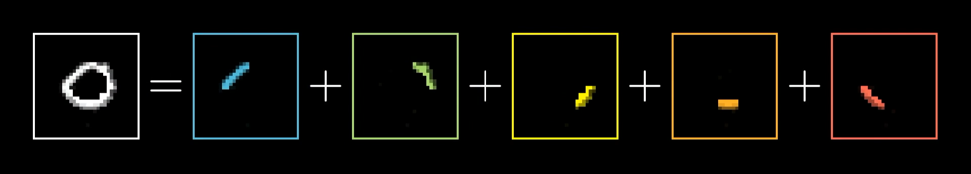
Image decomposition of a handwritten digit '0' into several edge components: diagonal, curve, and horizontal segments. Each colored box shows a different learned feature from the image.

🔍 Breaking Down Complexity

Digit "0" Analysis:

Top curve (red box)
Right edge (blue box)
Bottom curve (green box)
Left edge (yellow box)

🎯 The Insight

Complex shapes are combinations of simpler edges. If we can detect edges, we can detect shapes!

4 edges detected → Likely a "0"

More Edge Detection Examples

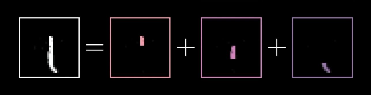
Image decomposition of a digit '1' into vertical and slightly slanted edges using learned features. Shows how a digit is built from simpler components.

🔍 Digit "1" Analysis

Simpler Pattern:

Main vertical line (blue)
Top angle (red)
Base extension (yellow)

🤔 Notice: Different digits require different types of edge detection. The network must learn to detect ALL possible edge types!

Scaling Up: Imagine doing this for every possible handwriting style, for every digit, automatically!

Beyond Digits: Universal Pattern Recognition

Side-by-side image showing a lion on the left and its corresponding edge-detected version on the right, used to explain how neural networks or vision systems detect edges.

🌍 Universal Applications

Edge Detection Works For:

Animal recognition
Face detection
Medical imaging
Satellite imagery
Quality control

🚀 Powerful Principle

The same hierarchical approach works across completely different domains!

                    This is why neural networks are revolutionary: One approach, infinite applications.
                

Hierarchical Processing in Other Domains

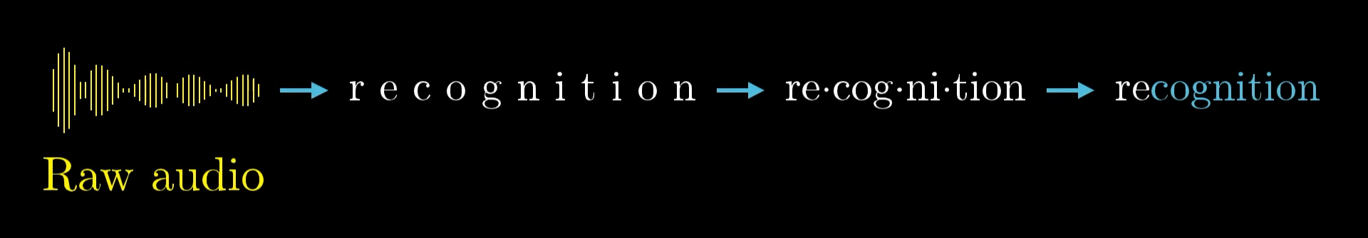
A visual of raw audio waveform transforming into the word 'recognition' through successive processing stages: audio ➝ text ➝ syllables ➝ final cleaned-up text. Demonstrates the transformation in speech recognition.

🎵 Speech Recognition Hierarchy

Layer by Layer:

Layer 1: Raw audio → Basic sounds
Layer 2: Sounds → Phonemes
Layer 3: Phonemes → Syllables
Layer 4: Syllables → Words
Layer 5: Words → Meaning

Complex Problem = Hierarchy of Simple Steps

Universal Truth: Most intelligent tasks can be broken down into hierarchical processing steps.

Part IV

The Mathematics: How Information Flows

🔗 Understanding Weights: The Connection Strength

Now we get to the heart of how neural networks actually work. The magic lies in the weights.

🧠 The Core Concept

A weight is simply a number that determines how much influence one neuron has on another. That's it.

Here's how it works:

Positive weight: "When the first neuron is active, the second should be active too"
Negative weight: "When the first neuron is active, the second should be inactive"
Zero weight: "These neurons don't influence each other"
Large magnitude: Strong influence (positive or negative)
Small magnitude: Weak influence

🎯 Analogy: Think of weights like volume controls. Some connections are turned up loud (high positive/negative), others are barely audible (near zero).

Weights in Action: Detecting a Specific Edge

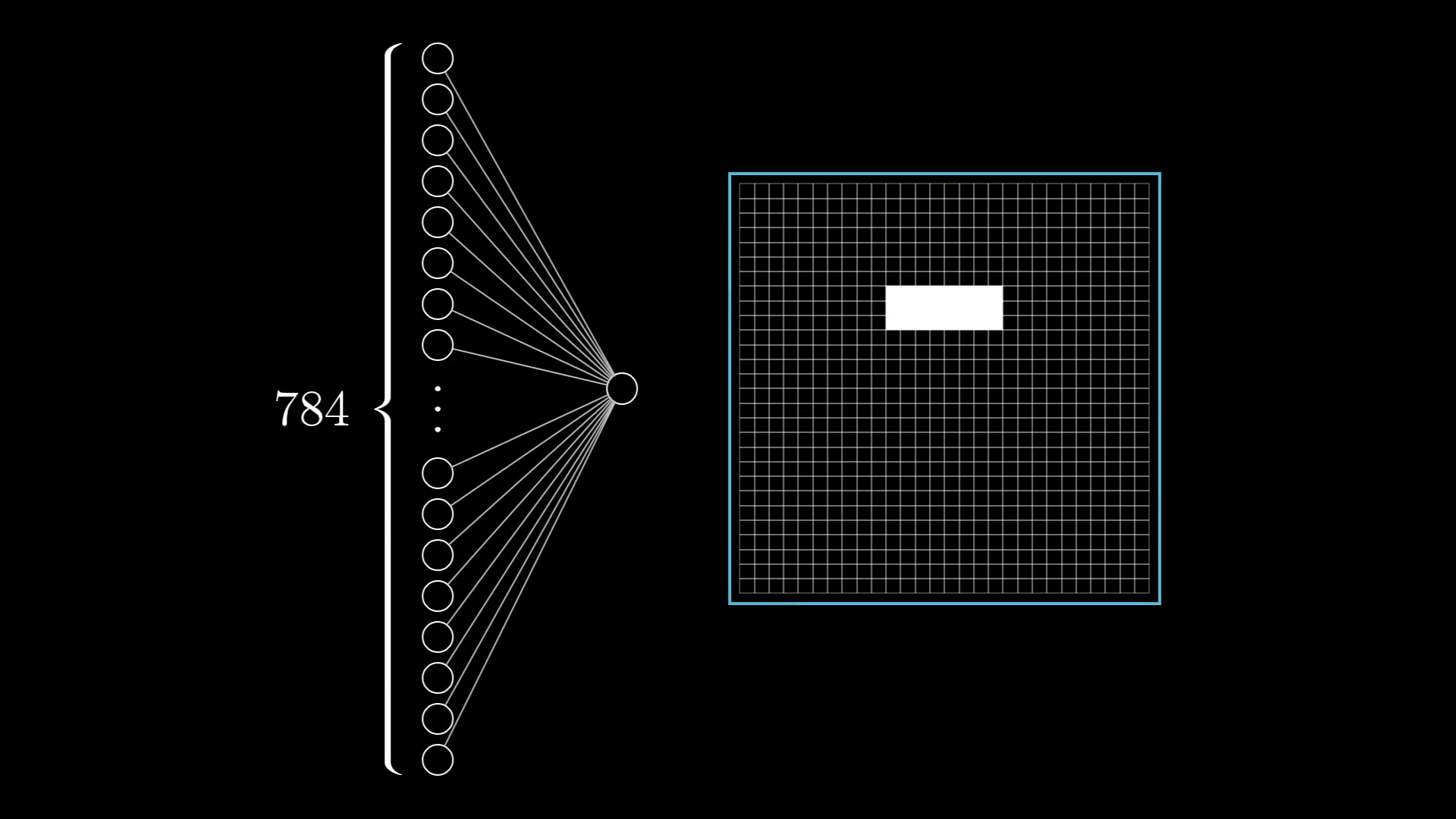
A neuron connected to a 784 input grid with a small white rectangle in the image. Demonstrates how a single neuron might detect a specific localized feature (like an edge) in an image.

🎯 The Goal

We want this neuron to detect this specific edge pattern.

Strategy:

High positive weights where we want bright pixels
High negative weights where we want dark pixels
Zero weights where we don't care

Response = Σ(weight × pixel_value)

💡 The Insight

By carefully choosing 784 weights, we can make this neuron respond strongly to our desired pattern and weakly to others!

Visualizing Weights: The Complete Picture

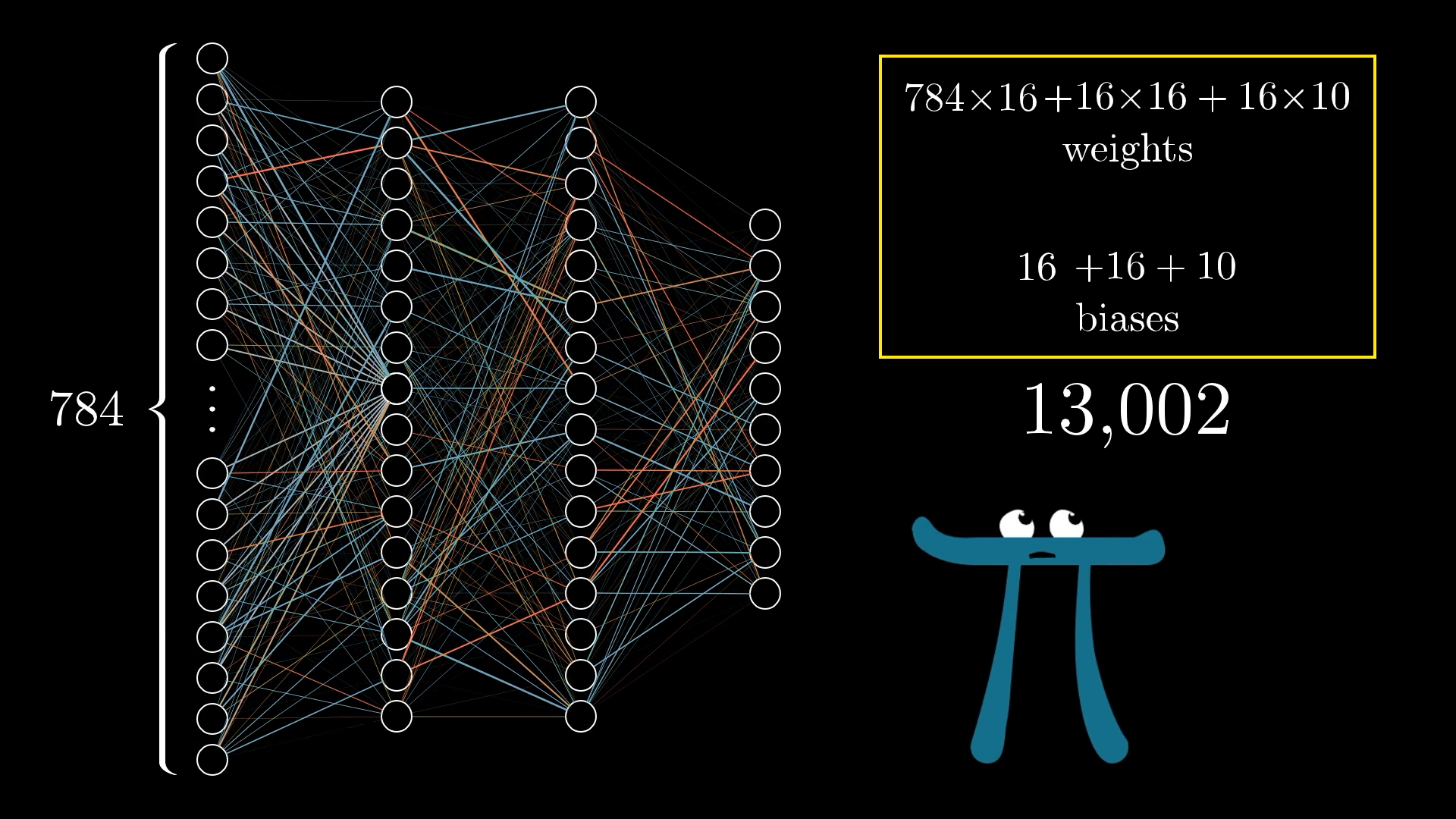
Fully connected neural network with weights shown in blue and red colors based on polarity. Side box breaks down the total number of weights and biases—13,002 in total.

📊 The Numbers

Weight Breakdown:

Input to Hidden 1: 784×16 = 12,544 weights
Hidden 1 to Hidden 2: 16×16 = 256 weights
Hidden 2 to Output: 16×10 = 160 weights
Plus biases: 16+16+10 = 42

Total: 13,002 parameters to learn!

⚠️ Complexity Alert: Each of these 13,002 numbers must be precisely tuned for the network to work!

🧮 The Weighted Sum: Core Calculation

Every neuron in a hidden or output layer performs the same fundamental calculation:

weighted_sum = w₁×a₁ + w₂×a₂ + w₃×a₃ + ... + wₙ×aₙ

Where:

wᵢ = weight of connection i
aᵢ = activation of neuron i in previous layer
n = number of neurons in previous layer

🎯 What This Means

Each neuron is asking: "Based on the pattern of activations in the previous layer, and given my weights, how excited should I be?"

🤔 Think About It: If a neuron has learned to detect horizontal lines, it will have positive weights for horizontally-aligned pixels and negative weights elsewhere.

Part V

Activation Functions: The Squishification

The Problem: Unlimited Range

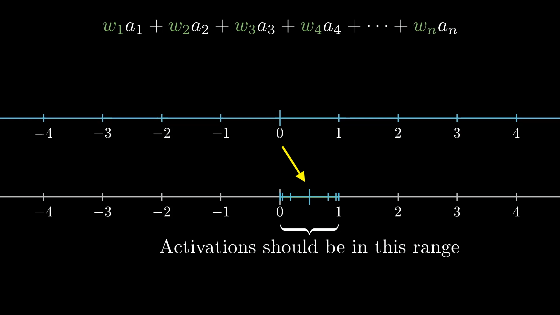
A number line with a yellow arrow pointing at the small region between 0 and 1, emphasizing that neural activations are squished into this range after applying an activation function like sigmoid.

⚠️ The Challenge

Weighted Sum Problems:

Can be any number: -1000, +500, etc.
Our neurons need values 0.0-1.0
Need smooth, differentiable function
Should preserve relative ordering

Need: ℝ → [0,1]

🎯 Requirements

We need a function that smoothly maps any real number to our desired 0-1 range, while preserving the relative magnitudes.

The Sigmoid Function: Perfect Solution

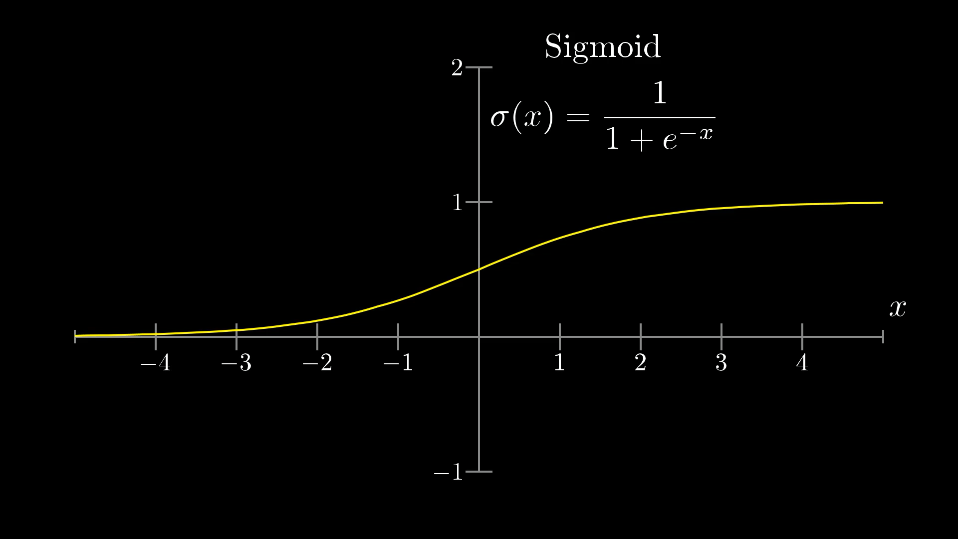
A graph of the sigmoid activation function: σ(x) = 1/(1 + e^(-x)). The curve transitions smoothly from 0 to 1 as x increases.

📈 Sigmoid Properties

Mathematical Definition:

σ(x) = 1/(1 + e^(-x))

Key Properties:

Range: (0, 1) - perfect for our needs!
Smooth and continuous
Differentiable everywhere
S-shaped curve
σ(0) = 0.5 (midpoint)

🧪 Test Your Understanding: What is σ(-1000)? Close to 0! What about σ(1000)? Close to 1!

Bias: Fine-Tuning Activation

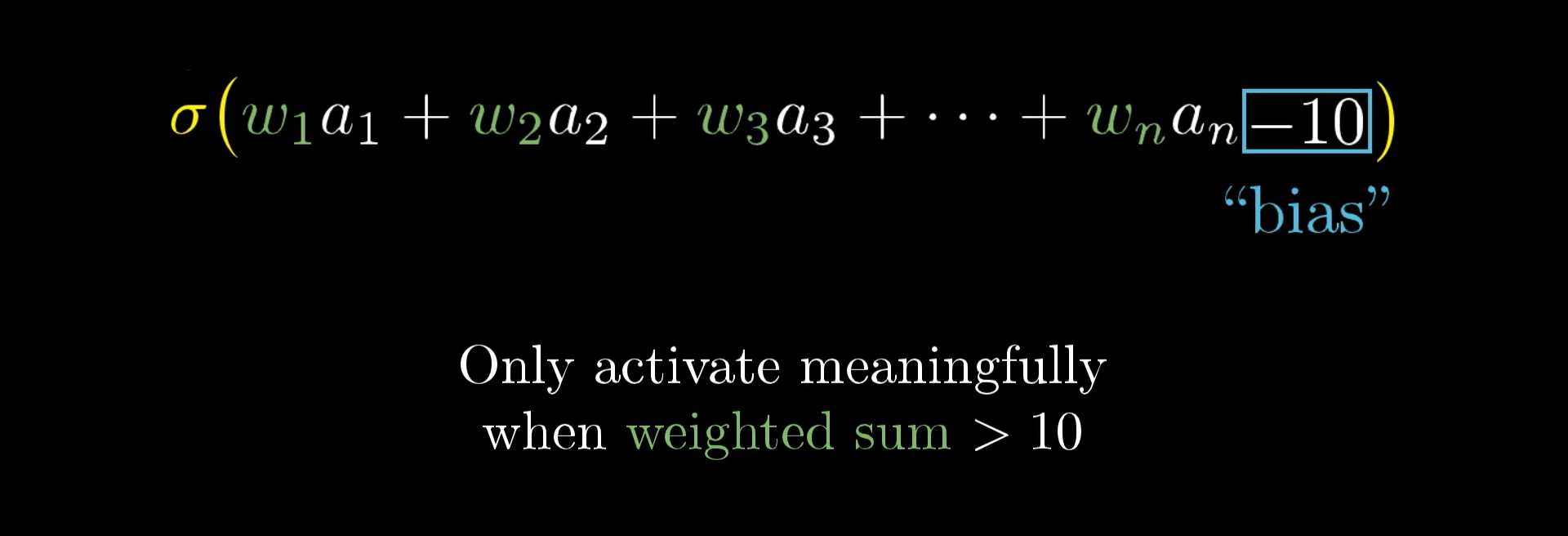
Mathematical expression with a highlighted negative bias (-10) and a caption stating that neurons only activate meaningfully when the weighted sum exceeds 10. Explains the role of bias in neural nets.

⚙️ The Role of Bias

Problem: What if we don't want the neuron to activate when weighted_sum > 0?

Solution: Add a bias term!

activation = σ(weighted_sum + bias)

Bias Effects:

Negative bias: Harder to activate
Positive bias: Easier to activate
Zero bias: Activates at weighted_sum = 0

🎯 Control Mechanism

Bias lets us control exactly when each neuron should "fire"!

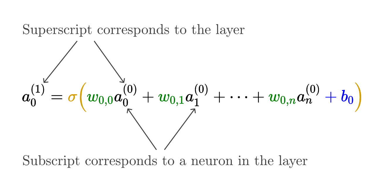
🧮 The Complete Neuron Formula

Now we can write the complete formula for any neuron's activation:

aⱼ = σ(w₁ⱼa₁ + w₂ⱼa₂ + w₃ⱼa₃ + ... + wₙⱼaₙ + bⱼ)

Where:

aⱼ = activation of neuron j in current layer
wᵢⱼ = weight from neuron i (prev layer) to neuron j (current layer)
aᵢ = activation of neuron i in previous layer
bⱼ = bias of neuron j
σ = sigmoid function

🎉 This is it!

This single formula describes how every neuron in every hidden and output layer computes its activation. The entire network is just this formula applied thousands of times!

                    Universal Truth: Despite all the complexity we've discussed, every neuron does exactly the same simple calculation!
                

Part VI

Matrix Mathematics: Elegant Notation

Matrix Magic: Computing All Neurons at Once

Annotated equation showing how activations are calculated in a neural network layer. Highlights how superscripts represent layers, subscripts represent neurons, and biases are added after weighted sums.

🧮 Matrix Power

Instead of computing each neuron individually, we can compute ALL neurons in a layer simultaneously using matrix operations!

a⁽ˡ⁺¹⁾ = σ(W⁽ˡ⁾a⁽ˡ⁾ + b⁽ˡ⁾)

Notation Guide:

a⁽ˡ⁾: Activations of layer l
W⁽ˡ⁾: Weight matrix from layer l to l+1
b⁽ˡ⁾: Bias vector for layer l+1
σ: Applied element-wise

📐 Matrix Dimensions: Getting the Math Right

Understanding matrix dimensions is crucial for implementing neural networks:

📊 Dimension Analysis

For a layer with n input neurons and m output neurons:

Weight matrix W: m × n (rows = outputs, cols = inputs)
Input activations a: n × 1 (column vector)
Bias vector b: m × 1 (column vector)
Output activations: m × 1 (column vector)

(m × n) × (n × 1) + (m × 1) = (m × 1)

Why This Matters:

Enables vectorized computation (much faster!)
Libraries like NumPy/TensorFlow optimize matrix operations
Makes code cleaner and more readable
Essential for implementing backpropagation (next lesson!)

🎯 Pro Tip: Always check your matrix dimensions when implementing neural networks. Dimension mismatches are the #1 source of bugs!

Part VII

The Big Picture: Understanding the Complete System

🔧 The Network as a Function

Let's step back and see the forest for the trees:

                    Fundamental Truth: A neural network is just a very complicated function that takes numbers as input and produces numbers as output.
                

For our digit recognizer:

Input: 784 numbers (pixel values)
Output: 10 numbers (digit probabilities)
Parameters: 13,002 weights and biases
Operations: Matrix multiplications and sigmoid applications

f(pixel₁, pixel₂, ..., pixel₇₈₄) = (prob₀, prob₁, ..., prob₉)

🤯 Mind-Blowing Realization

This "function" can recognize handwritten digits better than most humans, yet it's just arithmetic operations applied in sequence!

Sophisticated Solution for the Complexity

🔥 The Complexity/ Challange

13,002 parameters to tune
Thousands of multiplication operations
Non-linear transformations at each layer
Intricate interaction patterns
Emergent intelligent behavior

Fact: No human could ever manually set these 13,002 parameters to make the network work!

✨ The Solution

Every neuron follows the same simple rule
Just weighted sums and sigmoid functions
Beautiful mathematical structure
Scalable to any size network
Universal approximation capability

                    Note: Infinite complexity emerges from infinite repetition of simple operations!
                

🔮 How network Learn?

We now understand the structure and mathematics, but the biggest question remains:

The Question: How does the network learn the right values for those 13,002 parameters?

What we know so far:

✅ What neurons are and how they work
✅ How layers organize to solve complex problems
✅ How weights and biases control behavior
✅ How activation functions keep values in range
✅ How matrix math makes it all efficient

What we still need to learn:

❓ How do we find the right weight values?
❓ What does "learning from examples" actually mean?
❓ How do we measure if our network is improving?
❓ How do we automatically adjust thousands of parameters?

🎯 Next Topic

The learning process involves gradient descent and backpropagation - elegant mathematical techniques that automatically adjust all 13,002 parameters to minimize prediction errors!