πŸ” Local Search & Optimization

From Hill Climbing to Finding Global Solutions

Dr. Dhaval Patel β€’ 2025

πŸ” What Exactly is Local Search?

Local search is a fundamentally different approach to solving optimization problems. Unlike traditional search algorithms that maintain a frontier of unexplored nodes and systematically explore the entire search space, local search operates on a completely different principle.

Local search algorithms operate using only a single current node (not multiple paths) and generally move only to neighbors of that node.

Key Characteristics:

  • Single State Focus: Maintains only one current state at any time
  • Neighborhood Exploration: Only considers states reachable in one step
  • Path Irrelevant: Doesn't care how we got to current state, only where we are
  • Memory Efficient: Uses constant space regardless of problem size
  • Incomplete: May not find a solution even if one exists
  • Fast: Can find reasonable solutions quickly for large problems
Real-World Applications: VLSI design, job scheduling, neural network training, traveling salesman problem, facility location, and many AI optimization tasks where finding a "good enough" solution quickly is more valuable than guaranteeing the optimal solution.

πŸ”οΈ Why Use Local Search? The Mountain Climbing Analogy

Imagine you're a hiker trying to reach the highest point in a mountain range, but you're caught in thick fog that limits your visibility to just nearby terrain. This perfectly captures the essence of local search.

The Fog Analogy Explained:

  • Limited Visibility: You can only see immediate neighbors (one-step moves)
  • No Global Map: No complete knowledge of the entire landscape
  • Greedy Decisions: Always move to the highest visible point
  • Local Information: Make decisions based only on current surroundings
  • Risk of Local Peaks: Might reach a hill that's not the highest mountain
Key Insight: Sometimes we don't need the path to the solution - we just need to find the best state itself! The journey doesn't matter, only the destination.

When to Choose Local Search:

  • Large State Spaces: When systematic search would take too long
  • Optimization Problems: Finding best configuration rather than path
  • Continuous Spaces: Infinite or near-infinite search spaces
  • Time Constraints: Need reasonable solution quickly
  • Memory Limitations: Cannot store large search trees

🎯 Path-Finding vs. State Optimization: A Deep Dive

Path-Based Search

Goal: Find the sequence of actions to reach a goal state

"How do I get from A to B?"

Examples:

  • GPS Navigation: Find route from home to work
  • Puzzle Solving: Steps to solve Rubik's cube
  • Game Playing: Move sequence to win chess
  • Robot Planning: Actions to reach target location

What Matters: The sequence of moves, total cost of path, optimality of route

State Optimization

Goal: Find the best possible arrangement or configuration

"What's the best arrangement?"

Examples:

  • 8-Queens: Arrange queens so none attack
  • Scheduling: Assign tasks to minimize completion time
  • Circuit Design: Place components to minimize wire length
  • Portfolio Optimization: Allocate investments for best return

What Matters: The final configuration quality, not how we arrived there

VS

πŸ“Š Understanding Optimization Problems

Before diving into local search algorithms, we need to understand how to convert problems into optimization format. This is crucial because local search works on objective functions rather than goal tests.

Components of an Optimization Problem:

  • State Space: All possible configurations or solutions
  • Objective Function: Maps each state to a numerical value
  • Goal: Find state that maximizes (or minimizes) the objective function
  • Constraints: Rules that valid solutions must satisfy
Key Difference: Instead of asking "Is this a goal state?" we ask "How good is this state?"

Satisfaction vs. Optimization:

  • Constraint Satisfaction: Find any valid solution (like solving sudoku)
  • Constraint Optimization: Find the best valid solution (like best sudoku solution in minimum time)
  • Pure Optimization: All states are valid, just find the best one
Converting Problems: Many satisfaction problems can be converted to optimization by defining how many constraints are violated (minimize violations) or how many are satisfied (maximize satisfaction).

⛰️ Hill Climbing Algorithm

The Foundation of Local Search

πŸ₯Ύ Hill Climbing: Step-by-Step Breakdown

Hill climbing is the simplest and most intuitive local search algorithm. Think of it as a greedy algorithm that always takes the locally best step.

1

Initialize

Start with a random state or use problem-specific heuristics to choose a good starting point. This initial state becomes your "current" state.

2

Generate Neighbors

Find all neighboring states - states reachable by one legal move. The definition of "neighbor" depends on your problem domain.

3

Evaluate All Neighbors

Calculate objective function value for each neighbor. This tells us how "good" each potential move is.

4

Select Best Neighbor

Choose the neighbor with the best value (highest for maximization, lowest for minimization). If there are ties, choose randomly among the best.

5

Check Termination

If no neighbor is better than current state, STOP - you've reached a local optimum. Otherwise, move to the best neighbor and repeat from step 2.

function HILL-CLIMBING(problem):
    current ← MAKE-NODE(INITIAL-STATE[problem])
    loop do
        neighbor ← highest-valued successor of current
        if VALUE[neighbor] ≀ VALUE[current] then
            return STATE[current]
        current ← neighbor

β™› Understanding the N-Queens Problem

The N-Queens problem is a classic puzzle that perfectly demonstrates local search concepts. Let's start with the simpler 4-Queens version to understand the fundamentals.

N-Queens problem initial state showing 8 queens placed on a chessboard with string representation 16257483

Problem Definition:

  • Goal: Place N queens on an NΓ—N chessboard
  • Constraint: No two queens can attack each other
  • Attack Rules: Queens attack along rows, columns, and diagonals
  • Solution: Any valid arrangement satisfying all constraints
Why Start with N-Queens? The NΓ—N board is complex enough to demonstrate the key concepts of local search while being visualizable and understandable.

Understanding Queen Attacks:

  • Horizontal: Queens attack all squares in their row
  • Vertical: Queens attack all squares in their column
  • Diagonal: Queens attack along both diagonal directions
Key Insight: For N-Queens, we need exactly N queens placed such that each row, column, and diagonal contains at most one queen. The string representation shows queen positions as "16257483" where each position indicates the row of the queen in that column.

β™› The 8-Queens Problem: Optimization Approach

Now let's scale up to the classic 8-Queens problem and see how we convert this constraint satisfaction problem into an optimization problem suitable for local search.

8-Queens problem with heuristic calculations
Converting to Optimization Problem: Instead of finding any valid solution, we minimize the number of constraint violations.

Optimization Formulation:

  • State: All 8 queens placed on the board (one per column)
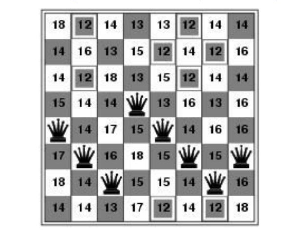
  • Objective Function h(n): Number of pairs of queens attacking each other
  • Goal: Minimize h(n) to reach h = 0 (perfect solution)
  • Neighbor Definition: Move one queen to different row in same column
Example: In the shown configuration, h = 17 attacking pairs. Our goal is to find moves that reduce this number, ideally to h = 0.

Why This Formulation Works:

  • Measurable Progress: Each move can be evaluated numerically
  • Local Improvements: Can make greedy decisions based on h-value
  • Clear Termination: h = 0 means we found a solution
  • Neighbor Generation: Easy to generate all possible single-queen moves

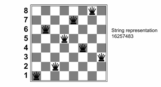
State Representation: We can represent each state as a string like "24748552" where position i contains the row number of the queen in column i.

πŸ”’ Hill Climbing on 8-Queens: Detailed Example

Let's walk through exactly how hill climbing works on the 8-Queens problem, step by step.

Starting Configuration Analysis:

Looking at our initial state with h = 17 attacking pairs:

  • Row Conflicts: Count queens in same row
  • Diagonal Conflicts: Count queens on same diagonal
  • Total Conflicts: Sum all attacking pairs
Neighbor Generation: For each of the 8 queens, we can move it to any of the other 7 positions in its column. This gives us 8 Γ— 7 = 56 possible neighbors.

Evaluation Process:

  • For each neighbor: Calculate new h-value
  • Compare values: Find minimum h among all neighbors
  • Make move: If best neighbor is better than current, move there
  • Repeat: Continue until no improvement possible
Computational Efficiency: We don't need to recalculate h from scratch each time. When moving one queen, we can incrementally update the conflict count by considering only the affected pairs.

Typical Hill Climbing Trajectory:

Starting from h = 17, a typical run might progress: 17 β†’ 12 β†’ 8 β†’ 5 β†’ 3 β†’ 2 β†’ 1 β†’ stuck at local minimum

🧠 Quick Check: Understanding Hill Climbing

Question: You're using hill climbing on 8-Queens and reach a state where all 56 possible moves result in worse or equal h-values compared to your current state (h = 2). What has happened?
A) Found the global optimum (h = 0)
B) Reached a local minimum (stuck)
C) Made a computational error
D) Need to generate more neighbors
Answer: B) Reached a local minimum (stuck)
Hill climbing stops when no neighbor is better than the current state. With h = 2, we haven't reached the global optimum (h = 0), but we're stuck at a local minimum where all single-queen moves make things worse. This is exactly why basic hill climbing only succeeds 14% of the time on 8-Queens!

⚠️ When Hill Climbing Gets Stuck

Understanding the Fundamental Limitations

πŸ—ΊοΈ The Hill Climbing Landscape: Understanding the Terrain

Before diving into specific problems, let's visualize the optimization landscape that hill climbing algorithms must navigate. This landscape metaphor helps us understand why local search can get stuck.

Hill climbing landscape showing global maximum, local maximum, shoulder, and current state with objective function plotted against state space
Key Landscape Features: The search space contains peaks (local maxima), flat areas (plateaus/shoulders), and valleys that create challenges for local search algorithms.
Search landscape showing all three types of problems: local maxima, plateaus with shoulders, and ridges that create challenges for hill climbing algorithms

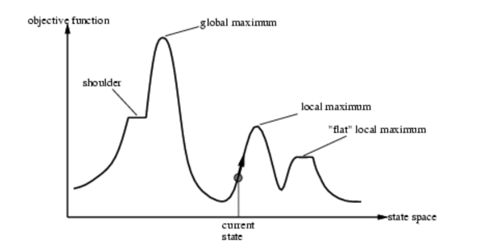
Understanding the Terrain:

  • Global Maximum: The highest peak - our ultimate goal
  • Local Maximum: Smaller peaks that can trap the algorithm
  • Shoulder: Flat areas that extend from peaks
  • Current State: Where our algorithm is currently positioned
  • State Space: All possible configurations we can explore
Navigation Challenge: Hill climbing can only see immediate neighbors, like navigating in thick fog where visibility is limited to just a few steps in any direction. The second image shows how all three problem types (local maxima, plateaus, and ridges) appear in the optimization landscape.

πŸ”οΈ Problem 1: Local Maxima

The Local Maximum Trap

A local maximum is a state that is better than all its neighbors, but not necessarily the best state in the entire search space.

Analogy: Like reaching the top of a small hill when Mount Everest is nearby but hidden by fog.

Why This Happens:

  • Limited Vision: Hill climbing only sees immediate neighbors
  • Greedy Nature: Always takes the locally best step
  • No Backtracking: Cannot undo previous moves

8-Queens Example:

Might get stuck at h = 1 (one attacking pair) where all single moves make things worse, even though h = 0 solutions exist.

Frequency: For 8-Queens, basic hill climbing gets stuck in local maxima about 86% of the time!

Characteristics of Local Maxima:

  • Optimization Trap: Algorithm terminates prematurely
  • Solution Quality: Often far from optimal solution
  • Predictable Failure: Same starting points lead to same local maxima
  • Problem Dependency: Frequency varies by problem structure

πŸ”οΈ Problem 2: Plateaus (Flat Areas)

The Plateau Problem

A plateau is a flat area of the search space where all neighboring states have the same objective function value.

Analogy: Like walking on a flat mesa where every direction looks the same height.

Two Types of Plateaus:

  • Flat Local Maximum: Flat area that is a local optimum
  • Shoulder: Flat area with better regions beyond it

The Challenge:

Standard hill climbing stops because no neighbor is better, but progress might be possible by moving to equally good states.

Solution Preview: Allow "sideways moves" to states with equal value, but limit the number to avoid infinite loops.

Plateau Characteristics:

  • Stagnation Risk: Algorithm stops making progress
  • Hidden Potential: Better solutions may exist beyond the flat area
  • Exploration Challenge: Need strategy to traverse flat regions
  • Infinite Loop Risk: Moving in circles without direction

Real-World Examples:

Plateaus commonly occur in neural network training when loss functions have flat regions, scheduling problems with equivalent arrangements, and game AI when multiple moves have equal evaluation scores.

πŸ”οΈ Problem 3: Ridges and Diagonal Movement

A ridge is a long, narrow area of high values with steep sides. The challenge is that progress along the ridge requires diagonal movement, but hill climbing can only move to direct neighbors.

Analogy: Like trying to walk along a narrow mountain ridge when you can only move north, south, east, or west - but the ridge runs northeast to southwest.

Why Ridges Are Problematic:

  • Limited Move Set: Can only make moves defined by neighbor function
  • Steep Sides: Any single step off the ridge leads to much worse states
  • Diagonal Progress: Optimal path requires coordinated multi-variable changes
  • Local Optima Chain: May get stuck at any point along the ridge

Real-World Example:

In neural network training, the loss function often has ridges where optimal progress requires adjusting multiple weights simultaneously, but gradient descent adjusts one dimension at a time.

Ridge Navigation: Advanced techniques like simulated annealing or genetic algorithms can better handle ridges by allowing coordinated multi-dimensional moves or accepting temporary downhill moves.

8-Queens and Ridges:

Ridges are less common in 8-Queens because the discrete nature of the problem and the neighbor definition, but they can occur in continuous optimization problems or problems with more complex neighbor relationships.

πŸ“Š Hill Climbing Performance: The Numbers

Let's examine the empirical performance of hill climbing on the 8-Queens problem to understand its strengths and limitations.

Experimental Setup: Run hill climbing from many random starting states and measure success rate and steps to solution.

8-Queens Performance Statistics:

  • Success Rate: 14% (finds solution h = 0)
  • Failure Rate: 86% (gets stuck at local minimum)
  • Steps When Successful: Average of 4 steps
  • Steps When Stuck: Average of 3 steps
  • Search Space Size: 8^8 β‰ˆ 16.7 million possible states
Remarkable Efficiency: When hill climbing works, it finds solutions incredibly quickly - just 4 steps on average in a space of 16 million states!

What These Numbers Tell Us:

  • Fast Convergence: Algorithm terminates very quickly (good or bad)
  • High Failure Rate: Most random starts lead to local optima
  • Predictable Failure: Usually fails within a few steps
  • Memory Efficient: Uses O(1) space regardless of search space size

Trade-off Analysis: Hill climbing trades completeness (guaranteed solution finding) for speed and memory efficiency. This trade-off is often worthwhile in real-world applications where "good enough" solutions are acceptable.

πŸ”§ Smart Solutions to Hill Climbing Problems

Escaping Local Optima

↔️ Solution 1: Allowing Sideways Moves

The simplest modification to basic hill climbing is to allow sideways moves - moves to neighbors with equal objective function values. This helps escape plateaus and shoulders.

Key Modification: Instead of stopping when no neighbor is strictly better, continue moving to equally good neighbors.

Algorithm Modification:

if VALUE[neighbor] ≀ VALUE[current] then
    // Original: stop here
if VALUE[neighbor] < VALUE[current] then
    // Modified: only stop if strictly worse

The Infinite Loop Problem:

  • Issue: Might move in circles on flat areas
  • Solution: Limit the number of consecutive sideways moves
  • Typical Limit: 100 sideways moves before giving up
8-Queens Results with Sideways Moves:
β€’ Success rate increases from 14% to 94%
β€’ Average steps for success: 21 steps
β€’ Average steps for failure: 64 steps

Trade-offs:

  • Pro: Dramatically improved success rate
  • Con: Takes longer to run (more steps per attempt)
  • Pro: Still very fast compared to systematic search
  • Con: Still gets stuck at local maxima (6% of the time)

🎲 Solution 2: Hill Climbing with Random Restarts

"If at first you don't succeed, try, try again!" This is the most practical and widely-used enhancement to hill climbing.

1

Run Basic Hill Climbing

Start from a random initial state and run hill climbing until it terminates (either finds solution or gets stuck).

2

Check Success

If hill climbing found a satisfactory solution, return it and stop. Otherwise, record the best solution found so far.

3

Generate New Random Start

Create a completely new random initial state, independent of previous attempts. This gives us a fresh perspective on the search space.

4

Repeat Process

Go back to step 1 and repeat the entire process. Continue until finding a solution or reaching a time/iteration limit.

Key Insight: Different starting points lead to different local optima. By trying many starts, we eventually find one that leads to the global optimum.
Mathematical Analysis: If each restart has probability p of success:
β€’ Expected number of restarts: 1/p
β€’ For 8-Queens with p = 0.14: Expected β‰ˆ 7 restarts
β€’ Total expected steps: 7 Γ— 4 = 28 steps

🚢 Solution 3: Hill Climbing with Random Walk

The Completeness Problem

Pure hill climbing can never be complete (guaranteed to find a solution if one exists) because it can get permanently stuck in local optima.

Random walk, on the other hand, is asymptotically complete - given infinite time, it will eventually find any reachable solution.

The Key Insight:

Combine the efficiency of greedy hill climbing with the completeness of random exploration.

The Hybrid Algorithm

At each step, make a probabilistic choice:

  • With probability p: Make greedy move to best neighbor (exploitation)
  • With probability (1-p): Move to a randomly chosen neighbor (exploration)
Parameter Tuning:
β€’ High p (e.g., 0.8): Mostly greedy, fast convergence
β€’ Low p (e.g., 0.3): More exploration, better escape from local optima

Benefits:

  • Escape Mechanism: Random moves can escape local optima
  • Maintains Progress: Greedy moves still drive toward better solutions
  • Tunable Balance: Can adjust exploration vs. exploitation

🎯 Solution 4: Stochastic Hill Climbing Variations

Instead of always choosing the single best neighbor, stochastic variations introduce randomness in the selection process while still biasing toward better moves.

Three Main Stochastic Approaches:

1. Stochastic Hill Climbing
Instead of choosing the absolute best neighbor, randomly select among the uphill moves, with probability proportional to the steepness of each move.

How it works: If we have neighbors with improvements of +2, +5, and +1, we might select them with probabilities 2/8, 5/8, and 1/8 respectively.

2. First-Choice Hill Climbing
Generate neighbors randomly (rather than systematically) and choose the first one that is better than the current state.

Advantage: Useful when the number of neighbors is very large, as we don't need to evaluate all of them.

3. Random-Restart Random Walk Hill Climbing
Combine all techniques: at each step, choose between greedy move, random move, or random restart.
Advanced Variation - Tabu Search: Keep a "tabu list" of recently visited states and forbid returning to them. This prevents cycles and encourages exploration of new areas.

Performance Considerations:

  • Diversification: Stochastic selection explores more of the search space
  • Robustness: Less likely to get trapped by single bad decision
  • Parameter Sensitivity: Performance depends on random number generation and probability distributions

πŸ”₯ Simulated Annealing: Physics-Inspired Search

🌑️ Cooling Metal to Perfect Crystal Structure

The Metallurgy Inspiration

Simulated annealing mimics the physical process of annealing in metallurgy - slowly cooling molten metal to form perfect crystal structures.

Physical Process:

  • High Temperature: Atoms move randomly, high energy
  • Gradual Cooling: Atoms settle into lower energy states
  • Slow Cooling: Allows time to find global minimum energy
  • Fast Cooling: Gets trapped in suboptimal crystal structure
Search Algorithm Mapping:
β€’ Energy β†’ Objective Function: Lower energy = better solution
β€’ Temperature β†’ Randomness: Higher temp = more random moves
β€’ Cooling β†’ Time: Gradually reduce randomness over time

🌑️ Simulated Annealing: Mathematical Foundation

Simulated annealing extends hill climbing by occasionally accepting moves that worsen the objective function, with the probability of acceptance decreasing over time.

Core Idea: Accept bad moves early (high temperature) to escape local optima, then become increasingly greedy (low temperature) to converge to optimum.

The Acceptance Probability Formula:

P(accept worse move) = e^(Ξ”E/T)
where:
β€’ Ξ”E = change in objective function (negative for worse moves)
β€’ T = current temperature (positive)

Understanding the Formula:

  • Ξ”E > 0: Better move β†’ always accept (probability = 1)
  • Ξ”E < 0: Worse move β†’ accept with probability e^(Ξ”E/T)
  • High T: e^(Ξ”E/T) β‰ˆ 1 β†’ accept most moves
  • Low T: e^(Ξ”E/T) β‰ˆ 0 β†’ reject most bad moves
  • Small |Ξ”E|: More likely to accept slightly bad moves
Temperature Schedule Examples:
β€’ Linear: T(t) = Tβ‚€ - Ξ±t
β€’ Exponential: T(t) = Tβ‚€ Γ— Ξ³α΅— (where Ξ³ < 1)
β€’ Logarithmic: T(t) = Tβ‚€ / log(1 + t)

Algorithm Steps:

  • Initialize: Start with high temperature T and random state
  • Generate Neighbor: Create random successor state
  • Calculate Ξ”E: Difference in objective function values
  • Accept/Reject: Always accept if better, probabilistically if worse
  • Cool Down: Reduce temperature according to schedule
  • Repeat: Continue until temperature reaches minimum or time limit

🧬 Genetic Algorithms: Evolution in Action

Instead of maintaining a single solution, genetic algorithms maintain a population of solutions and evolve them over generations using principles inspired by natural selection.

Initial position of N-Queens showing multiple random starting configurations for genetic algorithm population
Genetic algorithm workflow showing initial population, fitness function evaluation, selection, crossover, and mutation steps with numerical examples
🧬

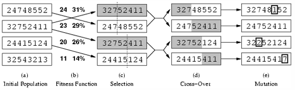
Population Initialization

Start with a diverse population of random solutions (typically 50-1000 individuals). Each solution is encoded as a string (like DNA). The first image shows various initial N-Queens configurations.

⭐

Fitness Evaluation

Evaluate each individual using a fitness function (opposite of cost function). Better solutions get higher fitness scores and higher reproduction probability.

πŸ‘₯

Selection for Reproduction

Choose pairs of parents for breeding based on fitness. Common methods: roulette wheel selection, tournament selection, rank-based selection.

πŸ”€

Crossover (Recombination)

Combine genetic material from two parents to create offspring. For strings, this might mean swapping segments at random crossover points.

⚑

Mutation

Randomly change small parts of offspring to maintain genetic diversity and explore new areas of the search space.

8-Queens Example: Represent each solution as string "24748552" where position i contains row of queen in column i. Fitness = 28 - (number of attacking pairs). The diagrams above show both the initial population diversity and how genetic operations work together through selection, crossover, and mutation phases.

🧬 Genetic Algorithm: 8-Queens Example

Let's see how genetic algorithms work on 8-Queens with a concrete example of one generation.

Population Representation:

Each individual is a string of 8 digits representing queen positions:

  • Individual 1: "24748552" (fitness = 24)
  • Individual 2: "32752411" (fitness = 23)
  • Individual 3: "24415124" (fitness = 20)
  • Individual 4: "32543213" (fitness = 11)
Fitness Function: fitness = 28 - (attacking pairs)
Maximum possible fitness is 28 (perfect solution), minimum is 0.

Selection Process:

Selection probabilities based on fitness:

  • Individual 1: 24/(24+23+20+11) = 31%
  • Individual 2: 23/78 = 29%
  • Individual 3: 20/78 = 26%
  • Individual 4: 11/78 = 14%

Crossover Example:

Parent 1: "24748552" | Parent 2: "32752411"

Crossover point after position 3:

  • Child 1: "247|52411" β†’ "24752411"
  • Child 2: "327|48552" β†’ "32748552"
Mutation: With small probability (e.g., 1%), randomly change one digit in each child. Example: "24752411" β†’ "24752413"

βš–οΈ Comparing Local Search Methods

Hill Climbing Variants

Best For: Quick solutions, limited resources

  • Basic HC: Fast, simple, 14% success
  • Sideways Moves: 94% success, more steps
  • Random Restarts: Nearly 100% success
  • Random Walk: Complete, tuneable
Simple to implement and understand

Advanced Methods

Best For: Complex problems, high-quality solutions

  • Simulated Annealing: Theoretically optimal
  • Genetic Algorithms: Population diversity
  • Tabu Search: Memory-guided exploration
  • Beam Search: Multiple parallel searches
More sophisticated but complex to tune
βš–οΈ

πŸŽ“ Final Challenge: Choosing the Right Algorithm

Scenario: You're working on a real-time optimization system that needs to find good (not necessarily optimal) solutions for scheduling problems in under 1 second, with limited memory. Which approach would you choose?
A) Basic hill climbing
B) Hill climbing with random restarts
C) Simulated annealing
D) Genetic algorithm
Answer: B) Hill climbing with random restarts
Given the constraints (real-time, limited memory, "good enough" solutions), random restarts provides the best balance: high success rate, predictable runtime, minimal memory usage, and easy implementation. It's the "Swiss Army knife" of local search - versatile, reliable, and practical for most real-world applications.

🎯 Complete Summary: Local Search Mastery

Core Principle: Local search trades completeness for efficiency, focusing on finding good solutions quickly rather than guaranteeing optimal solutions.

Algorithm Hierarchy (Simple β†’ Complex):

  • Basic Hill Climbing: Greedy local search, fast but often gets stuck
  • Hill Climbing + Sideways: Escapes plateaus, much better success rate
  • Random Restarts: Multiple attempts, practical gold standard
  • Random Walk: Probabilistic mix of greedy and random moves
  • Simulated Annealing: Temperature-controlled acceptance of bad moves
  • Genetic Algorithms: Population-based evolution with crossover and mutation

Problem Types and Best Methods:

  • Discrete Optimization: Hill climbing variants work well
  • Continuous Optimization: Gradient descent or simulated annealing
  • Combinatorial Problems: Genetic algorithms or specialized operators
  • Multi-Modal Landscapes: Random restarts or population methods
When to Use Local Search:
βœ“ Large search spaces where systematic search is impractical
βœ“ Optimization problems where path doesn't matter
βœ“ Time-critical applications needing quick solutions
βœ“ Memory-constrained environments
βœ“ Problems where "good enough" solutions are acceptable

Real-World Impact: These algorithms power machine learning training, circuit design, scheduling systems, game AI, financial optimization, and countless other applications where finding excellent solutions quickly is more valuable than guaranteeing perfect solutions slowly.

You now understand the foundations of modern optimization - from simple hill climbing to sophisticated evolutionary algorithms. These tools are essential for any AI practitioner tackling real-world optimization challenges!

Slide 1 of 22