๐Ÿง  Informed Search Algorithms

Making AI Smarter with Heuristics

Dr. Dhaval Patel โ€ข 2025

๐ŸŽฏ What We'll Learn Today

By the end of this tutorial, you'll understand how AI systems can search intelligently rather than blindly exploring every possibility.

  • Blind vs Informed Search: Why "being smart" about searching matters
  • Heuristics: How we give AI systems "intuition"
  • A* Algorithm: The gold standard of intelligent search
  • Real Applications: GPS navigation, game AI, robotics
๐Ÿ’ก Think of it like this: Would you rather find your keys by checking every possible location in your house, or by thinking about where you most likely left them?

๐Ÿ” The Search Problem

Understanding the Foundation

๐Ÿ—บ๏ธ What is a Search Problem?

Imagine you're planning a road trip from your city to another. You have:

๐Ÿ Simple Route Finding

Start
โ†’
City A
โ†’
City B
โ†’
Goal

Each step costs time, fuel, or distance

  • Initial State: Where you start (your current city)
  • Goal State: Where you want to end up (destination city)
  • Actions: What you can do (drive to connected cities)
  • Path Cost: How much each action costs (distance/time/fuel)
๐ŸŽฎ Search problems are everywhere: GPS navigation, puzzle solving, game AI, robot path planning, and even planning your daily schedule!

๐Ÿ‘๏ธโ€๐Ÿ—จ๏ธ Blind vs Informed Search

๐Ÿ˜ต Blind Search

Start
?
?
?
?
?
?
?
?
?

Explores systematically without direction

  • Breadth-First Search (BFS)
  • Depth-First Search (DFS)
  • Uniform Cost Search
โš ๏ธ Can be very slow and wasteful

๐Ÿง  Informed Search

Start
๐ŸŽฏ Best
โŒ Poor
โŒ Poor
๐ŸŽฏ Better
โญ Goal!

Uses knowledge to guide exploration

  • Greedy Best-First Search
  • A* Search (the champion!)
  • IDA* Search
โœ… Much faster and more efficient
VS

๐Ÿงญ What are Heuristics?

A heuristic is like giving an AI system "intuition" about how close it is to the goal.

Romania Map with Cities and Distances

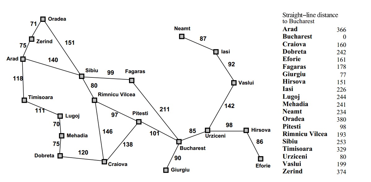
Romania Map - Our Classic AI Example

๐Ÿšซ Without Heuristics (BFS Problem)

Scenario: We are at Iasi and want to go to Oradea

Iasi โ†’ Neamt: cost = 87
Iasi โ†’ Vaslui: cost = 92

BFS chooses Neamt (87 < 92)

๐Ÿ”„ Problem: From Neamt, we can only return to Iasi!
Back at Iasi: same choice again โ†’ infinite loop!
Iasi โ†” Neamt โ†” Iasi โ†” Neamt...

๐ŸŽฏ With Heuristics (A* Solution)

Solution: f(n) = g(n) + h(n)

After returning from Neamt:
Total distance = 87 + 87 = 174
Now Vaslui is better choice!
โœ… A* considers both:
โ€ข g(n) = distance already covered
โ€ข h(n) = straight-line distance to goal
Prevents loops and guides toward goal!
  • h(n) = straight-line distance: Never overestimates actual road distance
  • Admissible heuristic: Optimistic but never too optimistic
  • Guides search: Towards promising directions, avoids loops
  • f(n) = g(n) + h(n): Balances past cost with future estimate

โญ A* Algorithm

The Gold Standard of Informed Search

๐Ÿงฎ The Magic Formula: f(n) = g(n) + h(n)

f(n) = g(n) + h(n)

g(n)

Cost so far

Actual cost from start to node n

Past Cost

h(n)

Estimated remaining cost

Heuristic estimate from n to goal

Future Estimate

f(n)

Total estimated cost

Complete path cost through n

Total Evaluation

๐Ÿ“ Example: From Arad to Bucharest

Sibiu

g(Sibiu) = 140

h(Sibiu) = 253

f(Sibiu) = 140 + 253 = 393

Timisoara

g(Timisoara) = 118

h(Timisoara) = 329

f(Timisoara) = 118 + 329 = 447

Zerind

g(Zerind) = 75

h(Zerind) = 374

f(Zerind) = 75 + 374 = 449

๐ŸŽฏ A* chooses Sibiu next (393 is lowest) because it has the best total estimated cost!

๐Ÿ‘ฃ A* Step-by-Step: Arad to Bucharest

Let's trace through A* finding the optimal path from Arad to Bucharest:

๐ŸŒณ A* Search Tree with f(n) = g(n) + h(n)

Step 1: Start at Arad
Arad
f = 0 + 366 = 366
Step 2: Expand Arad โ†’ Choose Sibiu (lowest f)
Sibiu
f = 140 + 253 = 393
Timisoara
f = 118 + 329 = 447
Zerind
f = 75 + 374 = 449
Step 3: Expand Sibiu โ†’ Choose Rimnicu Vilcea (lowest f)
Rimnicu Vilcea
f = 220 + 193 = 413
Fagaras
f = 239 + 176 = 415
Oradea
f = 291 + 380 = 671
Timisoara
f = 447
Zerind
f = 449
Step 4: Expand Rimnicu Vilcea โ†’ Choose Fagaras (f=415 < f=417)
Fagaras
f = 415
Craiova
f = 366 + 160 = 526
Pitesti
f = 317 + 100 = 417
Timisoara
f = 447
Step 5: Expand Fagaras โ†’ Choose Pitesti (f=417 < f=450)
Bucharest
f = 450 + 0 = 450
Pitesti
f = 417
Craiova
f = 526
Step 6: Expand Pitesti โ†’ GOAL!
Bucharest
f = 418 + 0 = 418 โœ“
Bucharest (Fagaras)
f = 450
๐Ÿ† A* finds optimal path: Arad โ†’ Sibiu โ†’ Rimnicu Vilcea โ†’ Pitesti โ†’ Bucharest (418 km)
๐ŸŽฏ Key insight: A* found Bucharest via Fagaras (450) but continued searching and found better path via Pitesti (418)!

๐Ÿง  Quick Understanding Check

Question: Why did A* choose Pitesti (f=417) over the Bucharest via Fagaras (f=450)?
A) Pitesti is closer to the start
B) A* always chooses the node with lowest f(n) value
C) Fagaras was already explored
D) Pitesti has a better heuristic
Answer: B) A* always chooses the node with lowest f(n) value
A* is systematic - it always expands the frontier node with the lowest f(n) = g(n) + h(n) value. Since Pitesti had f=417 and the Bucharest via Fagaras had f=450, A* chose Pitesti first. This led to finding a better path to Bucharest with cost 418!

โšก Why A* is Amazing: Key Properties

โœ… Complete

Always finds a solution if one exists

๐ŸŽฏ Optimal

Finds the best possible solution

๐Ÿš€ Efficient

Often much faster than blind search

โš ๏ธ Memory

Can use lots of memory

๐ŸŽฏ Admissible Heuristics

A heuristic h(n) is admissible if it never overestimates:

h(n) โ‰ค h*(n)
Romania Example:
โ€ข Straight-line Aradโ†’Bucharest: 366 km
โ€ข Actual road distance: 418 km
โ€ข Since 366 โ‰ค 418, it's admissible! โœ…

๐Ÿ“ Consistent Heuristics

Respects triangle inequality:

h(n) โ‰ค c(n,n') + h(n')
Romania Example:
โ€ข h(Arad) = 366
โ€ข c(Arad,Sibiu) = 140
โ€ข h(Sibiu) = 253
โ€ข Check: 366 โ‰ค 140 + 253 = 393 โœ…
๐Ÿ”‘ Key Insight: Admissible heuristics guarantee optimality because they're "optimistic" - they never overestimate the cost to reach the goal, so A* won't give up on the optimal path too early.

๐ŸŽ“ Advanced A* Techniques

๐Ÿ’พ IDA* (Iterative Deepening A*)

Problem: A* uses too much memory storing all nodes

Solution: Depth-first search with increasing f-cost limits

Romania Example:
Iteration 1: f-limit = 366 (start node)
Iteration 2: f-limit = 393 (next lowest f)
Iteration 3: f-limit = 413...
Continue until goal found
Trade-off: Uses O(bd) memory but may re-expand nodes

โšก Weighted A*

Formula: f(n) = g(n) + w ร— h(n), where w > 1

Effect: More greedy, faster but less optimal

Romania with w = 2:
Sibiu: f = 140 + 2ร—253 = 646
Timisoara: f = 118 + 2ร—329 = 776
Zerind: f = 75 + 2ร—374 = 823
โ†’ Still choose Sibiu, but more greedy
Trade-off: Solution cost โ‰ค w ร— optimal cost
๐ŸŽฏ Real-world tip: Many GPS systems use weighted A* with w โ‰ˆ 1.5 to get "good enough" routes quickly, especially for real-time applications with changing traffic conditions.

๐ŸŒ A* in the Real World

A* isn't just academic - it powers technologies you use every day!

๐Ÿ—บ๏ธ GPS Navigation

๐Ÿ“ฑ

Google Maps, Apple Maps

  • Find shortest routes
  • Avoid traffic
  • Real-time re-routing

๐ŸŽฎ Video Game AI

๐Ÿ•น๏ธ

NPC Pathfinding

  • Character movement
  • Enemy AI behavior
  • Strategic planning

๐Ÿค– Robotics

๐Ÿค–

Robot Navigation

  • Warehouse automation
  • Self-driving cars
  • Mars rovers

๐Ÿงฉ Puzzle Solving

๐Ÿงฉ

15-Puzzle, Rubik's Cube

  • Optimal puzzle solutions
  • Game strategy
  • Planning problems
๐Ÿš€ NASA used A* for Mars rover pathfinding! The rovers use it to navigate safely around obstacles on the Martian surface.

๐ŸŒณ Depth-First Branch & Bound

Systematic Optimal Search

๐ŸŽฏ DFBB Problem: Find Optimal Path A to G

Let's solve a classic problem: Find the optimal (shortest) path from node A to node G.

DFBB Problem Graph showing nodes A through G with edge costs

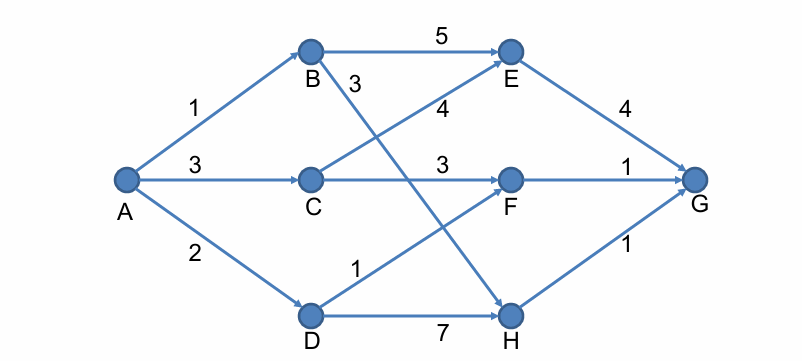
Problem Graph: Find shortest path from A to G

๐ŸŽฏ Goal: Find the path from A to G with minimum total cost using Depth-First Branch & Bound
  • Branch: Generate paths systematically using DFS
  • Bound: Use upper bound to prune suboptimal branches
  • Optimal: Guaranteed to find the shortest path
  • Systematic: Never expands the same node twice

๐Ÿ“Š Edge Costs Summary

From A:
Aโ†’B: 1, Aโ†’C: 3, Aโ†’D: 2
From B:
Bโ†’E: 5, Bโ†’C: 3
From C:
Cโ†’E: 4, Cโ†’F: 3, Cโ†’D: 1
From D:
Dโ†’H: 7
From E:
Eโ†’F: 4, Eโ†’G: 4
From F:
Fโ†’H: 1, Fโ†’G: 1
From H: Hโ†’G: 1

๐ŸŒณ DFBB Search Tree Exploration

Depth-First Branch & Bound systematically explores all paths while pruning suboptimal branches.

DFBB Search Tree showing complete exploration

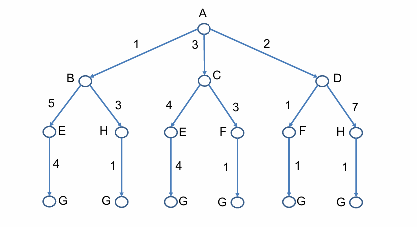
Complete Search Tree Structure

DFBB step-by-step exploration with pruning

Step-by-Step Exploration with Pruning

๐Ÿ” DFBB Process Summary

๐ŸŒณ Complete Search Tree:
1. Start at A (cost = 0)
2. Expand A โ†’ B, C, D
3. Choose B first (cost = 1)
4. From B โ†’ E (cost = 6), C (cost = 4)
5. Continue systematic exploration
6. Terminate expanding nodes when bound exceeded
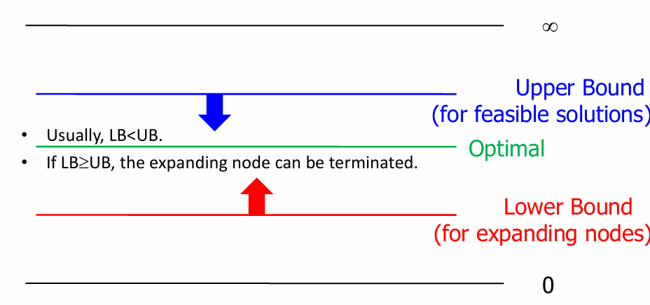
โœ‚๏ธ Bound-based Pruning:
โ€ข Usually UB < UB (Upper Bound improves)
โ€ข If UB > UB, the expanding node can be terminated
โ€ข For feasible solutions: update bounds
โ€ข For expanding nodes: compare with current bound
โ€ข Optimal path found when all branches explored or pruned
๐Ÿ† DFBB systematically explores the complete search tree while using bounds to prune suboptimal branches
๐ŸŽฏ Key insight: Upper bound guides pruning decisions - when current path cost exceeds best known solution, terminate that branch
โšก Efficiency: DFBB guarantees optimal solution by exploring all promising paths while eliminating provably suboptimal branches early!

๐Ÿ“Š DFBB: Upper and Lower Bounds

๐Ÿ“ˆ Branch & Bound Mechanism

Upper Bound (for feasible solutions)

Best complete solution found so far

UB

Updates when better complete path to goal is found

Provides pruning threshold for ongoing search

Lower Bound (for expanding nodes)

Minimum cost estimate for partial path

LB

Cost accumulated so far + optimistic estimate to goal

If LB โ‰ฅ UB, this path cannot be optimal

๐Ÿ” DFBB Termination Rule:

IF UB โ‰ฅ UB (bound comparison) THEN Expanding node can be terminated โœ‚๏ธ
Feasible Solutions:
Complete paths to goal G
Update Upper Bound if better
Enable more aggressive pruning
Update UB โœ“
Expanding Nodes:
Partial paths being explored
Compare bound with current UB
Terminate if cannot improve
Prune if LB โ‰ฅ UB โœ‚๏ธ

๐ŸŽฏ DFBB vs A*

  • Both optimal: Find best solution
  • DFBB: Systematic, never re-expands
  • A*: Uses heuristics, can be faster
  • DFBB: Uses less memory (DFS)

๐Ÿ’ก Key Insights

  • Upper bound: Gets better over time
  • More pruning: As UB improves
  • Optimal guaranteed: Systematic exploration
  • Memory efficient: O(bd) space

๐ŸŽ“ Key Takeaways

๐Ÿ† Smart search algorithms use knowledge (heuristics) or systematic exploration (bounds) to find optimal solutions efficiently!

๐Ÿง  A* Algorithm

f(n) = g(n) + h(n)

  • Uses heuristics
  • Optimal with admissible h(n)
  • Very efficient
  • High memory usage

๐ŸŒณ DFBB Algorithm

Branch + Bound

  • Systematic exploration
  • Always optimal
  • Low memory usage
  • Can be slower

๐ŸŽฏ When to Use

  • A*: Good heuristics available
  • DFBB: Memory constrained
  • Both: Need optimal solutions
  • Neither: "Good enough" is OK
๐Ÿ’ก The key insight: Being smart about search isn't just about speed - it's about using the right tool for the right problem. Heuristics guide us when we have good intuition, bounds help us when we need to be systematic!

๐Ÿ† Final Challenge

Scenario: You're building a robot navigation system for a warehouse. The robot needs to find the shortest path while avoiding obstacles. You have two options:

Option A: A* with Euclidean distance heuristic
Option B: Depth-First Branch & Bound

Which would you choose and why?
A) A* - faster with good heuristic
B) DFBB - uses less memory
C) A* - better for dynamic environments
D) Both are equally good
Answer: A) A* - faster with good heuristic

For robot navigation, A* is typically better because:
โ€ข Speed matters: Robots need real-time responses
โ€ข Good heuristics: Euclidean distance works well for physical spaces
โ€ข Dynamic replanning: Can quickly recompute when obstacles change
โ€ข Memory: Modern robots have sufficient memory for most warehouse scenarios

DFBB would be chosen only if memory was extremely limited or if we couldn't design a good heuristic.

๐ŸŽ‰ Congratulations!

You now master Informed Search Algorithms

Ready to build smarter AI systems! ๐Ÿค–โœจ

๐Ÿš€ Next: Implement A* and DFBB yourself!

๐ŸŽฏ Challenge: Design heuristics for new domains

๐ŸŒŸ Explore: Game AI, robotics, planning applications

Slide 1 of 20